Interactive Visualization of Vegetation Reflectance Models (IVVRM)

About

The Interactive Visualization of Vegetation Reflectance Models (IVVRM) tool is an interactive reflectance modelling environment mainly focusing on the Prospect + Sail (PROSAIL; Jacquemoud et al. 2009) radiative transfer model (RTM) family. All code, including the spectral models themselves, is written in Python allowing a time-efficient computation and a progressive visualization of the results whenever parameter settings, sensor options or model members are changed by the user. Main fields of application of the IVVRM tool are seen in education and training, particularly for students and PhD candidates who focus their research on vegetation remote sensing data analysis. The plasticity of the tool contributes to a better and faster understanding of the benefits and limitations of RTMs. Effects of changes in the concentration of diverse plant constituents become apparent especially in the accumulative plotting mode, where several parameters can be set independently and are visualized with relatable colors in a common plotting canvas for a local sensitivity analysis. Moreover, the IVVRM tool can be used as a starting point for hyperspectral data analysis. A manual adjustment of biophysical leaf and canopy parameters with the aim to minimize deviations between modelled and measured spectra serves as a simple but didactically clear inversion approach. Such an analysis extends the capability of the model by the knowledge of the user and allows for a more specific interpretation of the underlying processes in the transfer of incident radiation and the biophysics of vegetation. Improved understanding of the model dynamics for different vegetation types may facilitate the choice of more sophisticated methods, like iterative optimization algorithms, LUT-inversions or machine learning applications for biophysical variable retrievals (Verrelst et al. 2015).

Getting Started

In order to use IVVRM, the EnMAP-Box 3.0 or higher needs to be downloaded and properly installed as QGIS-plugin. Please visit EnMap-Box 3 documentation for further instructions on how to install and link EnMAP-Box 3.0 with QGIS. IVVRM is found in the Application menu item -> Agricultural Applications -> Interactive Visualization of Vegetation Reflectance Models (IVVRM). The tool will open a new window with default settings (Figure 1).

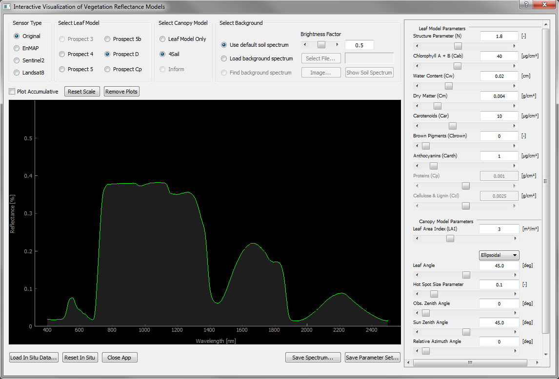
Figure 1: Screenshot of the Interactive Visualization of Vegetation Reflectance Models (IVVRM) main window with default settings.

Changing the input or post-processing settings of the model automatically invokes a new model run. The result is plotted in the black graph widget.

User Input

Sensor Type

By default, PROSAIL calculates reflectances with a spectral sampling width of 1 nm (original). If a different sensor type is selected, PROSAIL results are spectrally resampled to match the number and wavelengths of bands of specific sensors (currently: EnMAP hyperspectral imager, Sentinel-2 multispectral imager, Landsat-8 operational land imager). The spectral response function of those observation systems are supplied with the tool and might change after the actual launch of EnMAP. Reflectances for the central wavelengths of all sensor bands are calculated as weighted averages of neighboring PROSAIL output bands.

Tip

The resampling is a mathematical intensive process and takes longer than the actual model run. The more bands a target sensor comprises, the more inertly the tool will behave. Move the parameter sliders slowly when displaying model results as pseudo-EnMAP spectra (242 bands).

Leaf Model

For the leaf optical properties model, the user can choose from a variety of Prospect models, starting with Prospect 4 and the newest official version being Prospect D (Féret et al. 2017). Prospect Cp is a modification by Wang et al. (2015), splitting Dry Matter content into Proteins (CP), Cellulose & Lignin (Ccl) and dry residuals (Cm). Depending on the selected model, input parameters will automatically be enabled or disabled. An overview of the Prospect parameters and the versions they first appeared in, is given in Table 1.

Canopy Model

If wanted, Prospect can be coupled with a canopy architecture model to form top of canopy spectra. Up to now, only one version of SAIL (Scattering of Arbitrarily Inclined Leaves) – 4SAIL (Verhoef et al. 2007) – can be selected which will enable the Canopy Model Parameters (Table 1) section. For forestry application, the Invertable Forest Reflectance Model (INFORM) is considered for implementation and will then pose an alternative for model coupling.

Table 1: Overview of the PROSAIL parameters and their according dimensions, as used in the IVVRM tool. Some parameters, like e.g. the leaf chlorophyll content, are used in all Prospect versions, whereas other parameters were included in newer releases.

Parameter	Description	Unit	Model versions
N	Leaf structure parameter	-	Prospect (all)
Ccab	Leaf Chlorophylla+b content	µg cm-2	Prospect (all)
Cw	Leaf Equivalent Water content	cm	Prospect (all)
Cm	Leaf Mass per Area	g cm-2	Prospect (all)
Ccar	Leaf Carotenoids content	µg cm-2	Prospect 5
Cbr	Fraction of brown leaves	-	Prospect 5B
Canth	Leaf Anthocyanins content	µg cm-2	Prospect D
LAI	Leaf Area Index	m2 m-2	4SAIL
LIDF	Leaf Inclination Distribution Function	-	4SAIL
ALIA	Average Leaf Inclination Angle	deg	4SAIL
Hspot	Hot Spot size parameter	-	4SAIL
soil	Soil Reflectance (optional)	-	4SAIL
Psoil	Soil Brightness Parameter	-	4SAIL
SZA	Sun Zenith Angle	deg	4SAIL
OZA	Observer Zenith Angle	deg	4SAIL

Spectral background

When observing canopies instead of single leaves, information about the spectral background is required. By default, PROSAIL provides one typical bright and one typical dark soil spectrum, characterizing low and high moisture levels of the soil surface. The final background signal is computed using a soil brightness factor (Psoil), which can be defined by the user. A high value for Psoil gears towards the bright, a low value towards the dark soil spectrum.

If available, an individual background spectrum can be supplied via Load background spectrum (see chapter 4.2). In this case, the default SAIL background spectrum is overwritten and Psoil becomes obsolete. This is especially useful if in situ measurements of the open soil are available for the desired study area.

In the future, it is planned to select background spectra directly in the EnMAP-Box to reproduce an observation contained in a hyperspectral image.

Input parameters

On the right hand side of the window, input parameters are located and grouped into Leaf Model Parameters (Prospect) and Canopy Model Parameters (SAIL). Each group can be collapsed to save space. If the list is still longer than the vertical extent of the window, a scroll bar will automatically appear.

A parameter is changed either by moving its horizontal slider, or by entering the value directly in the text field and hitting return. Both approaches are limited by min and max values to prevent math errors or implausible model results. Every time a model parameter is changed, the reflectance model is re-calculated and the spectrum is updated and shown in the graph widget.

One special case of parameter is the Leaf Angle. Here, the user can choose between two different leaf angle distribution functions: ellipsoidal or beta-distribution. The ellipsoidal distribution function asks for an average leaf inclination angle which has to be supplied by the user in the respective text field. If a beta distribution is chosen, the field becomes disabled and a distribution function type is selected from the dropdown menu instead. Learn more about leaf inclination distribution function types in Goel & Strebel (1984).

Working with the tool

Navigating in the graph widget

The graph widget is a canvas with black background in which the model results are plotted. To be precise, it is a QGraphWidget provided through the QGIS framework and PyQt. This widget can be used interactively, allowing the user to change appearance and display settings on the fly. The following interactions are possible:

• Zooming in & out via mouse wheel

• Moving the graph by holding down left mouse button or mouse wheel and “dragging” the plot in the desired direction

• Specifying ranges for the axes via right click -> X-Axis (/ Y-Axis) -> Manual min & max

• Optimizing both axes ranges via right click -> View All

• Toggle grid lines on / off via right click -> Plot Options -> Grid

In addition, ranges for X-axis and Y-axis is set back to default by hitting Reset Scale (push button, located above the graph widget) and plots can be removed by clicking on Remove Plots (next to Reset Scale).

Importing in situ and background spectra

Whenever the push button Load In Situ Data… or Select File… in the background selection is clicked, a child window will appear (Figure 2).

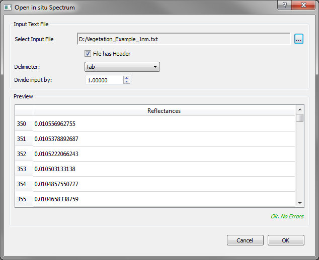
Example of the OPEN Dialog in IVVRM. The same dialog is used for in situ spectra and background model spectra. A file has to be selected and the reader will automatically find out whether the file has a header and which delimiter is used to separate data columns. A division factor can be set to put model output and file input on the same scale. If no errors occur, the user can proceed with the import.

In this dialog, at first an input file (in situ or background) has to be selected (only .csv or .txt allowed). The path will be shown in the sunken label section. IVVRM will inspect the file and automatically check if the first row is a header or not and will guess the delimiter according to the most frequent appearance in the file. If this information is sufficient to read the file correctly, its content will be displayed in the Preview-section. The user can manually override header information and delimiter and check if the file is still readable. A status message in the lower right corner will indicate possible errors. Only if there are no errors, the OK button is enabled and the user can proceed to the next step. Sometimes reflectances are given as multiples of a fraction of one, so that they can be stored using integer data type. A reflectance value of 5,000 would e.g. mean 50% or 0.5. To compare these data on different scales, a division factor can be set by the user. For the example mentioned, a division factor of 10,000 would put both data on the same scale.

Tip

If a text file cannot be read, although delimiter and header type are correct, you can check on the proper construction of the file by comparing with one of the example files in the application folder.

After confirming the text file, the user is directed to another dialog in which bands can be (de-)selected for/from processing (Figure 3). Multiple bands can be selected and moved to the list of excluded / included bands at once. When opening an In Situ Spectrum, the excluded bands will be set to Python “NaN” value. In the graph widget, data gaps will be substituted by a straight line between valid neighbor data points, but they are ignored in the statistics. For background spectra, data gaps are visualized the same, but the data points are in fact interpolated values that serve as valid input for the SAIL model.

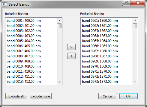
Figure 3: Single bands or ranges of bands can be excluded from the statistics of in situ and modelled spectra. For background spectra, the according wavelengths are interpolated linearly.

A default selection of bands / wavelengths is excluded or interpolated (Table 2). The according bands are filled into the exclusion and inclusion list.

Table 2: Default ranges for exclusion from statistics (in situ spectrum) or for interpolation (background signal)

Band range	Wavelength range [nm]	Domain
961 – 1021	1360 – 1420	Atmospheric water absorption
1391 – 1551	1790 – 1950	Atmospheric water absorption

If a spectrum text file consists of more than two columns, the first one is considered to supply wavelengths in nanometers and the others contain reflectance data. A mean value is calculated for each band in this case. In situ spectral data is removed from the graph widget and from statistics when Reset In Situ is clicked. For a reset of background spectra, the radio button in the Select Background frame needs to be moved to Use default soil spectrum. IVVRM will forget about the loaded spectra after each reset.

Tip

ASCII files with multiple columns representing multiple spectra can be created with ASD ViewSpec Pro, the data processing tool for ASD field spectrometers. In the ASCII Export section check Output to a Single File. The resulting text file is readable in IVVRM.

Statistical indices

When an In Situ Spectrum is successfully loaded into the graph widget, IVVRM will try to compare reflectances of the modelled vs. measured spectrum band-wise. If both spectra have the same number of bands, statistics are computed and the result is showed in the upper right corner of the graph widget. If the number of bands differs, a sensor mismatch is assumed, but the spectrum will still be displayed. The following statistical indices are calculated: Root Mean Squared Error (RMSE, Eq. (1)), Mean Absolute Error (MAE, Eq. (2)), Nash-Sutcliffe Efficiency (NSE, Eq. (3)), modified Nash-Sutcliffe-Efficiency (mNSE, Eq. (4)) and the Coefficient of Determination (R², Eq. (5)).

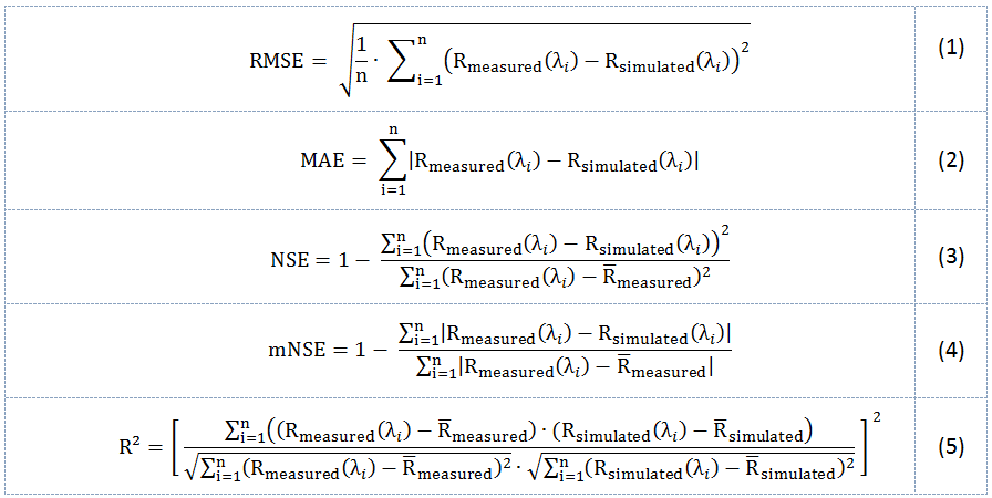
R_measured (λ_i) is the measured and R_simulated (λ_i) the modelled reflectance at wavelength λ for the i-th spectral sensor band. n is the total number of bands analyzed.

The statistics module is only active when accumulative plotting is switched off.

Exporting spectra and parameter sets

The export buttons, both located on the lower right of the graph widget, allow capturing current model inputs and outputs. Save Spectrum exports the currently modelled reflectances as text files with two data columns: wavelength and reflectance. They are built such that they can be re-loaded into IVVRM via Load In Situ Data. If a constellation of biophysical input parameters is found, it can be stored by clicking on Save Parameter Set. Only those parameters will be saved, however, that are used by the currently selected model.

Tip

Statistical indices can be used to approximate modelled and measured spectra until a suitable match is found. Next, the parameter constellation can be saved to finish a simple variable retrieval via manual optimization.

Accumulative plotting

The Plot Accumulative option is a check box above the upper left corner of the graph widget. It is disabled by default, so each call of PROSAIL overwrites the result of the previous model run and draws a graph in green. If accumulative plotting is selected, results are in turn stored and new plots are added to the existing one(s) with a parameter-specific style. The color of each plot is associated with a single parameter and indicates which of them had been changed to invoke the latest model run.

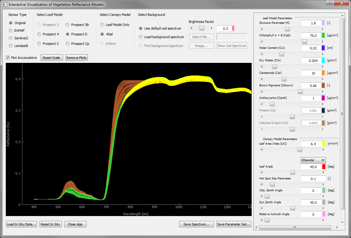
Figure 4: Accumulative plotting is enabled, so each biophysical model parameter is additionally labelled with a certain color. This color is in turn used for the graph whenever the parameter was changed to invoke a new model run. In this case, Cbr was increased stepwise from 0.0 to 0.66, then LAI was increased from 4.0 to 6.4 m2m.2 and finally Ccab was increased from 40 to 75 µg cm-2.

Not only is this option suitable to track changes of the biophysical input parameters (e.g. for a local sensitivity analysis), but also changes between different sensor types. They are depicted by different line styles (see Figure 5 and Table 3)

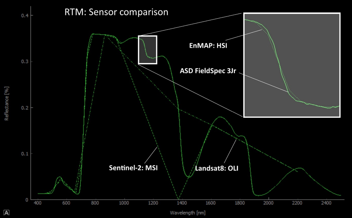
Figure 5: Another application of the accumulative plotting mode of IVVRM is the comparison of different spectral resolutions associated with different earth observation systems. Model output is displayed in different line styles for different sensors. Currently, four sensors are taken into account: solid (original model resolution, corresponds to most field spec sensors), dotted (EnMAP hyperspectral), dashed (Sentinel-2 multispectral) and dash-dot (Landsat8 multispectral). Hyperspectral resampling best reproduces the original shape of the PROSAIL output.

Table 3: Overview of spectral resampling to different sensor types and the line styles they are shown in for accumulative plotting.

Sensor Type	Line Style
Original (PROSAIL)	line
EnMAP hyperspectral	dotted
Sentinel2 multispec.	long dashed
Landsat 8 multisoec.	long dashed/dotted

Even though it looks like more plots are just being added to the canvas, they are all redrawn each time a new spectrum member comes in. For this reason, the tool becomes slower when too many spectra are contained in the graph widget, so it seems useful to remove the plots from time to time via Remove Plots.

References

Féret, J.B.; Gitelson, A.A.; Noble, S.D.; Jacquemoud, S. Prospect-d. Towards modeling leaf optical properties through a complete lifecycle. Remote Sensing of Environment 2017, 193, 204-215.

Goel, N. S. and D. E. Strebel. Simple beta distribution representation of leaf orientation in vegetation canopies. Agronomy Journal 1984, 76(5), 800-802.

Jacquemoud, S.; Verhoef, W.; Baret, F.; Bacour, C.; Zarco-Tejada, P.J.; Asner, G.P.; François, C.; Ustin, S.L. Prospect + sail models: A review of use for vegetation characterization. Remote Sensing of Environment 2009, 113, Supplement 1, S56-S66.

Verhoef, W.; Jia, L.; Xiao, Q.; Su, Z. Unified optical-thermal four-stream radiative transfer theory for homogeneous vegetation canopies. IEEE Transactions on Geoscience and Remote Sensing 2007, 45, 1808-1822.

Verrelst, J.; Camps-Valls, G.; Muñoz-Marí, J.; Rivera, J.P.; Veroustraete, F.; Clevers, J.G.P.W.; Moreno, J. Optical remote sensing and the retrieval of terrestrial vegetation bio-geophysical properties – a review. Isprs J Photogramm 2015, 108, 273-290.

Wang, Z.; Skidmore, A.K.; Wang, T.; Darvishzadeh, R.; Hearne, J. Applicability of the prospect model for estimating protein and cellulose+lignin in fresh leaves. Remote Sensing of Environment 2015, 168, 205-218.