Creation and Inversion of Look-up-tables
Creation of Look-up-tables
About
The creation of Look-up-table (LUT-create) tool enables an easy creation of a large set of simulated vegetation reflectance spectra according to given parameter ranges. Just as IVVRM, LUT-create mainly focuses on the Prospect + Sail (PROSAIL; Jacquemoud et al. 2009) radiative transfer model (RTM) family.
User Input
LUT-create demands the same presettings as IVVRM User Input
Getting Started
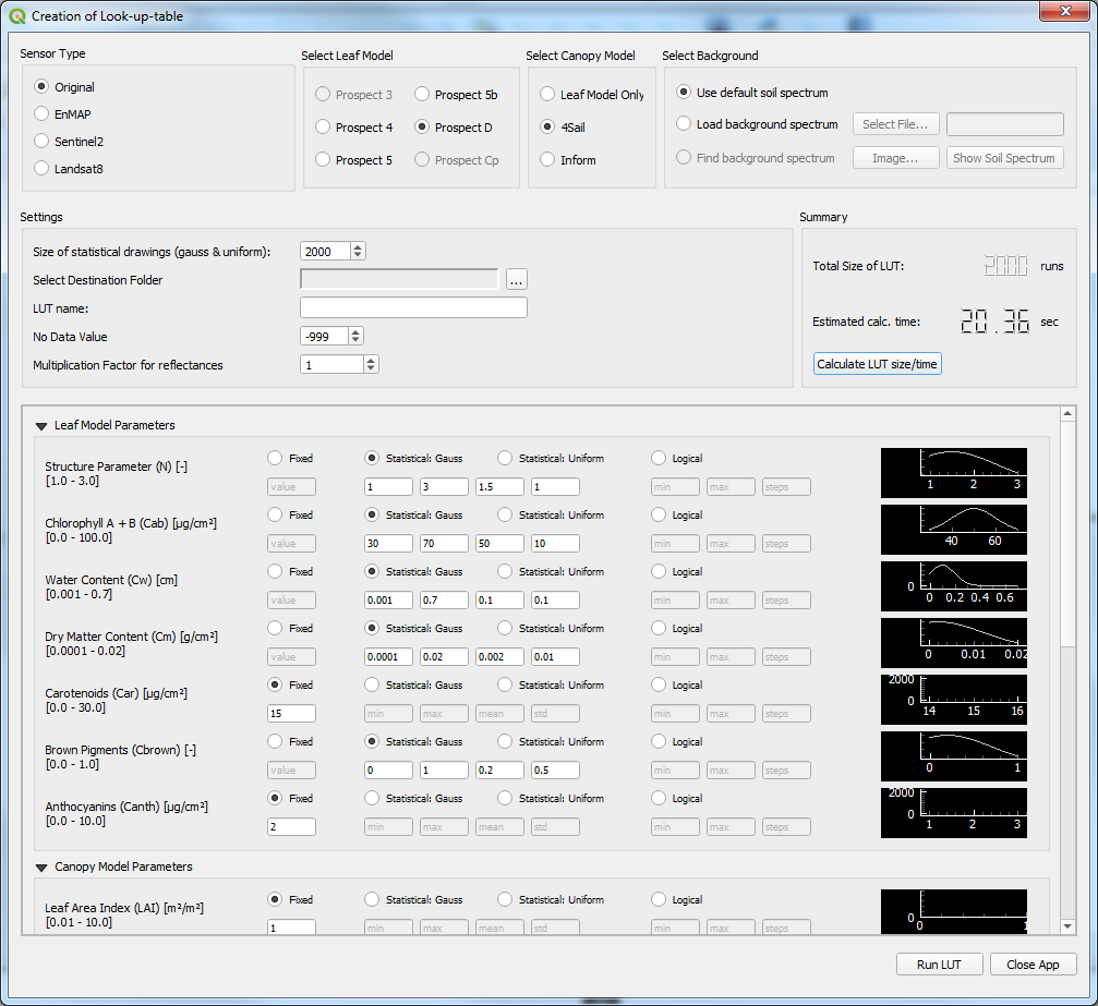
Figure 1: Screenshot of the Creation of Look-up-table main window with some defined parameter ranges.
Settings
Size of statistical drawings (gauss & uniform): Defines the number of statistical drawings according to the set ranges i.e.: Setting a number of 1000 and a gaussian range for Chlorophyll A + B (Min: 30; Max: 70; Mean: 45; SD: 10), the LUT will be filled with 1000 Chlorophyll-Values, following this distribution.
Select Destination Folder: the directory where the LUT will be written to.
LUT name: the file name of the LUT
No Data Value: standard no data value,… can be ignored since modelled spectra are continuous.
Multiplication factor for reflectances: By default, single spectra will be saved as floating point reflectance percentages. A multiplication by i.e. 10000 will be memory saving for very large look-up-tables (+- 50.000 members with logical distributed parameters) since output format will be integer.
Model Parameter Range Settings
The single Prospect & Prosail parameters per released version are described in the IVVRM Leaf Model and Canopy Model Section
Permitted parameter ranges can be found in brackets under the single parameters.
Parameter drawing probabilities:
Fixed: If a parameter is set to ‘fixed’, the parameter will have the same value in each modelled spectrum based on the number of statistical drawings.
Statistical: Gauss: The parameter will be gaussian distributed according to the min/max and the mean/standard deviation values. The distribution function determines the probability of a parameter value to be drawn. Once set, the gaussian distribution function will be plotted in the plot canvas to the right.
Statistical: Uniform: The parameter will be distributed uniformly according to the min/max value. Between min/max the probability of a parameter value to be drawn remains the same. Once set, the uniform distribution function will be plotted in the plot canvas to the right.
Logical: For each parameter that is set to be distributed logically, an additional look-up-table will be created according to the given number of steps. I.e. if different look-up-tables need to be created with regard to different sun zenith angle (SZA) conditions, SZA can be logically distributed.
Warning
Setting a parameters distribution to logical increases both the calculation time and the size of the LUT exponentially. It is not recommended to logically distribute more than one parameter.
Size/time estimation
Click Calculate LUT size/time to be able to estimate the calculation time in relation to the selected settings. If the calculation time appears to be too high, check if logically distributed parameters can be avoided.
Run
When input/output directives and all parameter ranges have been set click Run LUT to start the LUT-creation. After the creation has been finished the LUT consists of a meta data file (…_00meta.lut) and the LUT as a numpy array file .npy (…_0_0.npy only if LUT does not contain logical distributed parameters and has a maximum size of statistical drawings of 50.000)
Inversion of Look-up-tables
About
The Global Inversion of LUT (LUT-invert) tool enables the inversion of look-up-tables previously created via the LUT-create tool. For a given input reflectance raster the tool searches a set of best fitting simulated spectra from the LUT to conclude on the underlying parameters of the measured input spectra.
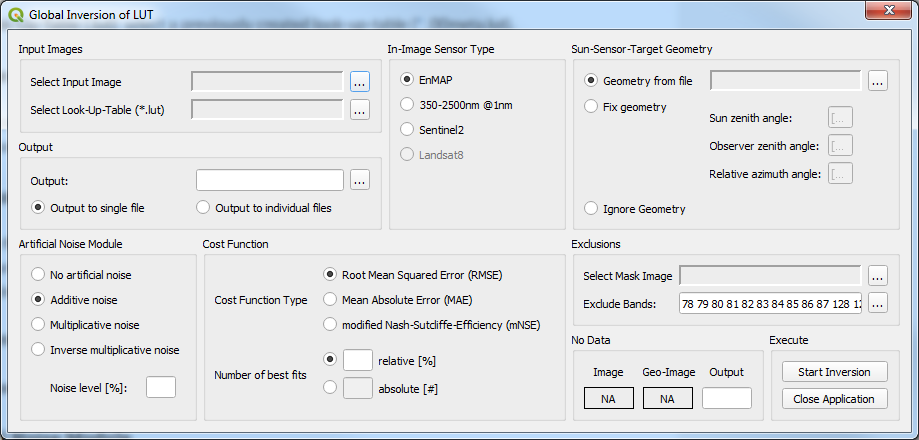
Figure 2: Screenshot of the Global Inversion of LUT main window.
User Input
Input Images
Select Input Image: import a GDAL readable raster with reflectance information.
Select Look-Up-Table (.lut): select a previously created look-up-table (_00meta.lut).
In-Image Sensor Type
The selected sensor type must match both the reflectance input raster and the sensor type selected for the LUT-creation.
Sun-Sensor-Target Geometry
Geometry from file: import a GDAL readable 3-Band raster with sun-sensor-target information: - Band 1: sun zenith angle (SZA) [deg] - Band 2: Observer/view zenith angle (OZA) [deg] - Band 3: relative azimuth angle (rAA) between the sensor and the sun [deg].
Fix geometry: set fixed values for the whole image
Ignore Geometry: do not take sun-senor-target angles into account (not recommended).
Artificial Noise Module
Since simulated spectra (in the LUT) are generally smoother than in situ measured spectra, adding artificial noise to the LUT spectra helps to improve comparability between the two data sets. Artificial noise will generally only be applied to the LUT spectra. Different calclulation methods (additive, multiplicative, inverse multiplicative) can be applied. The strengh of the artificial noise has to be adjusted in the Noise level [%] text field. A standard procedure consists of adding 4% additive noise.
Cost Function
Cost Function Type: choose the objective function what will be minimized in the search process. RMSE, MAE and mNSE can be selected.
Number of best fits: Depending on the number of spectra contained in the selected LUT, a relative [%] or a absolute number of best fitting spectra are taken into account for the calculation of the average underlying Prosail parameters. Allowing for only one best fitting spectrum, the result might be ill-posed due to unrealistic parameter combinations which unintentionally build up a well fitting spectrum. Setting a too large number, a too large range of parameters is averaged, concealing a clear signal of correct parameters.
Exclusions
The manual exclusion of bands from the analysis is a measure to focus on specific wavelength/band regions in the inversion process. I. e. if only pigment concentrations (Chlorophyll, Anthocyanins and Carotenoids) are of interest, the NIR and SWIR regions can be excluded from the analysis.
By default wavelengths lower than 400 nm, and the water vapor absorption bands between 1358-1477 nm and 1720-1998 nm are excluded from the analysis.
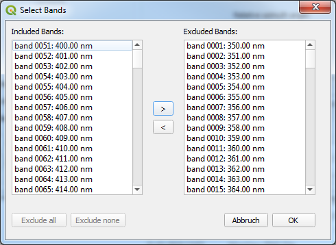
Figure 3: Screenshot of the Band Exclusion window.
No Data
The tool automatically detects the no data value/data ignore value of the input raster. It is highly recommended, that a no data value has been assigned to the input data so that the appropriate pixels are omitted by the algorithm. For this reason it is obligatory to also insert a output no data value in the corresponding text field.
Execute
When all inputs have been assigned click Start Inversion to begin global inversion of leaf and canopy parameters from measured spectra.