Manual Retrieval of Vegetation Variables using IVVRM

In the following tutorial we will retrieve vegetation biophysical and biochemical variables from a measured field spectrum using the IVVRM tool.

Aims:

• Understanding of how vegetation interacts with radiation and specificially how the different vegetation variables influence reflectance and absorbance in different spectral regions of the optical domain.

• Understanding of the diversity of vegetation reflectance signatures and the information they contain.

• Understanding of PROSPECT leaf and SAIL canopy radiative transfer models and their input - output parameters.

• Understanding of model parameter equifinality and its implications for variable retrieval.

Introduction

Note

For a thorough understanding of the content presented in this tutorial it is recommended to read the IVVRM Manual beforehand.

IVVRM uses a coupled vegetation radiative transfer models (RTM) scheme: The optical properties of leaves are represented by the PROSPECT model family, whereas the interaction of radiation with the whole canopy is characterized by the canopy reflectance models 4SAIL and INFORM. Employing the coupled models (=PROSAIL or INFORM+PROSPECT), a vegetation canopy reflectance spectrum can be simulated based on physical laws. Due to this physical basis, structural, biophysical and biochemical properties of a reflectance spectrum can be estimated by means of different model inversion strategies. This implies, if vegetation reflectance is measured either using a field spectrometer, airborne or spaceborne acquisitions, the absorption processes that lead to a specific recorded shape of a spectrum can be traced back by simulating a matching spectrum using for instance the PROSAIL model. RTM inversion strategies can be physically-based by using iterative optimization or Look up tables (LUT). Increasingly machine learning regression algorithms are applied that use the LUT as training data base and thus avoiding the collection of in situ calibration data. IVVRM only allows manual inversion, which is not physically-based but aims to increase the understanding of the different contributions and interactions of the diverse input parameters: Absorption areas of the vegetation constituents can be directly observed during the manual fitting process.

Starting IVVRM and import an in-situ spectrum

1. Start the IVVRM tool: go to the Applications tab in the EnMap-Box 3 main window.

2. From the Agricultural Applications choose Interactive Visualization of Vegetation Reflectance Models (IVVRM).

3. After clicking Start IVVRM the main window shows up with default settings.

4. Click on Load In Situ Data… and click on … in the Open in situ Spectrum window.

5. Select the file example_winterwheat_20180615_1nm.txt and click OK

6. In the Select Bands window confirm with OK again. By default the water vapor absorption bands are excluded.

In the IVVRM plot canvas you should now see the loaded in-situ spectrum in grey and the startup default simulated spectrum in green. The imported spectrum shows the spectral signature of a winter wheat canopy. It was recorded on June 15 in 2018 at 10:45 CEST with a handheld field spectrometer (ASD FieldSpec3) in an agricultural field north east of Munich, Germany (Coordinates: 48.247952 N, 11.715958 E).

As you might notice in the plot canvas, the in-situ spectrum and the simulated spectrum do not match which is also shown by the different error measures colored in blue in the plotted textbox. Currently IVVRM should look like Figure 1:

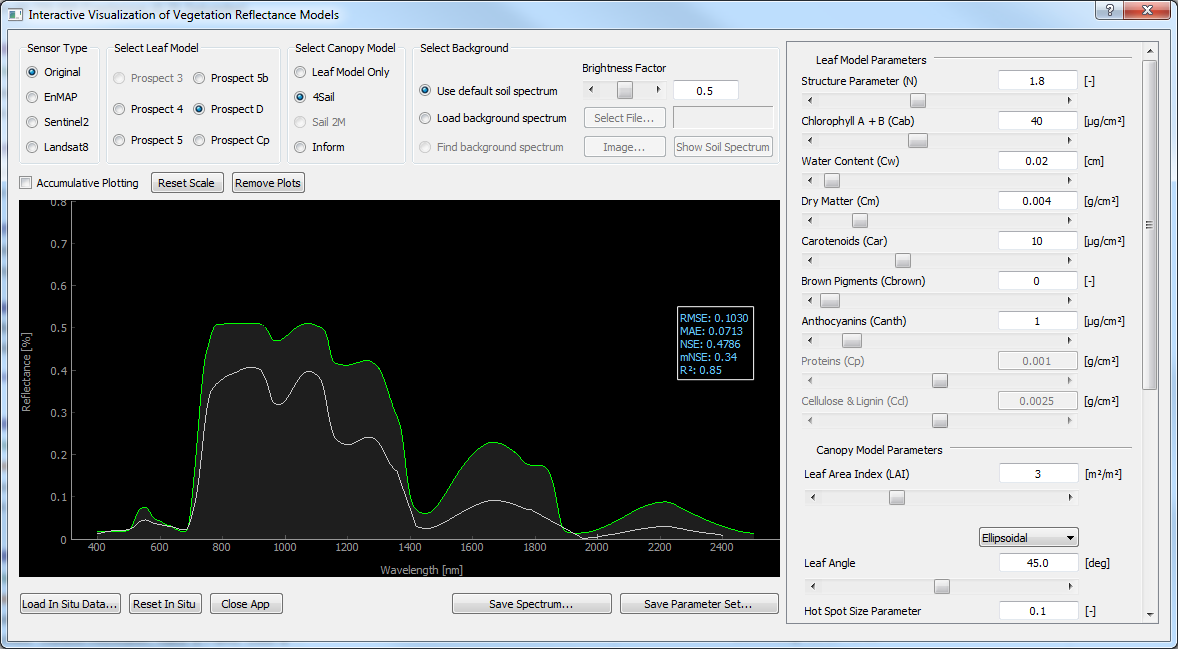
Figure 1: IVVRM with imported in-situ measured spectrum and default settings.

Fitting the spectra

In the next step we will try to fit these spectra manually. To achieve this we will keep the default settings in the frame above the plot canvas:

• Sensor Type: Original (Field Spectrometer)

• Select Leaf Model: Prospect D

• Select Canopy Model: 4Sail

• Select Background: use default soil spectrum @ Brightness Factor = 0.5 (see IVVRM-Manual for details)

Focus on the leaf and canopy model parameters to the right and try to adjust the slider positions with the aim that both spectra match as perfectly as possible. Every slider change triggers an instantaneous recalculation of the PROSAIL model.

Tip

As you move the sliders, observe in which wavelength ranges a parameter becomes absorption effective. Activate the Checkbox Accumulative Plotting, move the sliders, and get an idea of overlapping parameter sensitivities.

While trying to match the spectra consider the following:

How might a wheat canopy look like in a humid mid latitude environment in mid June and how might its biophysical/biochemical traits be pronounced at that time? Check Figure 2 below to get a more concrete impression of the conditions.

Figure 2: Picture of the winter wheat canopy on 15th June 2018 when spectra were measured.

Below you will find some help to better assess the conditions:

• Chlorophyll A + B content (Cab): Since ears are already well developed, the wheat is in its reproductive developing stage. Leaf chlorophyll content should still be on a high level before onset of senescence (between 50 and 65 µg cm^-2). Mind that not only Cab influences absorption in the visible (VIS) part of the spectrum. Try to fit carotenoid and anthocyanin content as well.

• Leaf Area Index (LAI): The higher the total leaf area the higher its reflectance in the near infrared (NIR) between 800 and 1300 nm. LAI should be around 4.5 and 6.5 m² m^-2.

• Leaf Angle (ALIA): This is a highly sensitive parameter. The higher the leaf inclination angle, the less radiation will hit the leaves to be then reflected by the soil surface.

• Sun-Sensor-Geometry: Imagine the light conditions at ~48° North in mid June at 10:45 CEST. The sun zenith angle (SZA) was approx. 40° (60° elevation angle). Since the sensor was held perpendicular to the surface (nadir measurement) both observer zenith angle (OZA) and relative azimuth angle (rAA) between sensor and target should be kept at 0°.

The remaining parameters were intentionally not addressed! While changing the sliders, try to minimize the error measures until you think your fitted result can not be improved anymore.

Click Save Parameter Set… to write your current parameter set to a text file.

Compare the result

Parallel to the spectroscopic measurements several vegetation variables have been measured in the field. Check Table 1 and compare the values of your best fit with the ones measured in June 2018. Mind that not all variables could be measured!

Focus on leaf chlorophyll content, leaf water content, leaf dry matter content, LAI, and ALIA. How close are your results to the measured values? Some of your results might be close while some might be far off.

Table 1: List of in-situ measured winter wheat variables on June 15th 2018

Parameter	Description	Measured
N	Leaf structure parameter	-
Ccab	Leaf Chlorophylla+b content	53.2
Cw	Leaf Equivalent Water content	0.07
Cm	Leaf Mass per Area	0.00441
Ccar	Leaf Carotenoids content	-
Cbr	Fraction of brown leaves	0.01
Canth	Leaf Anthocyanins content	-
LAI	Leaf Area Index	5.4
LIDF	Leaf Inclination Distribution Function	-
ALIA	Average Leaf Inclination Angle	61°
Hspot	Hot Spot size parameter	-
Psoil	Soil Brightness Parameter	-
SZA	Sun Zenith Angle	40°
OZA	Observer Zenith Angle	0°
rAA	rel. Azimuth Angle	0°

Use measured input data

Now use all the available measured variables as model input parameters!

The result should be close to the one shown in Figure 3:

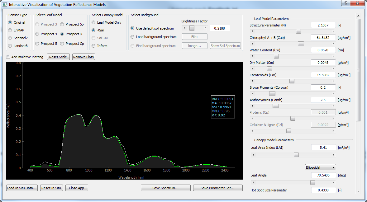
Figure 3: Using measured vegetation variables as input parameters for PROSAIL with slight adjustments for a best fit.

The modelled spectrum you see now might be similar to the one you created when trying to fit the spectra with little prior knowledge.

The issue we encounter here is called equifinality:

Equifinality (or the ill-posed nature) of models is a fundamental issue in environmental modelling. Any physically-based numerical model that consists of various input parameters to simulate any kind of environmental system is governed by equifinality: many different parameter sets may be equally valid in terms of their ability to reproduce an observed measured state.

When we invert RTMs to retrieve vegetation variables from a measured spectrum, many parameter combinations might result in the same spectrum. The scientific task lies in finding the most plausible one. This is achieved by using automatic retrieval schemes like for instance machine learning regression algorithms (MLRAs) or look-up-table inversion (LUT inversion). Here, not a single best fitting spectrum is accepted as true but a whole ensemble which is internally rated by an algorithm.

The presented tutorial on manual inversion using IVVRM emphasizes how the different vegetation constituents and their interactions affect the reflectance of a vegetation spectrum. Such exercises may increase the understanding of the complex processes occurring between solar radiation and vegetated surfaces and thus might help to improve and optimize parameterization when physically- based inversion of RTMs for the estimation of quantitative vegetation traits is carried out.